RESEARCH REPORT | Census Undercount | December 2022
UNDERCOUNTING AND OVERCOUNTING POPULATION IN TEXAS COUNTIES
A methodology for estimating the undercount in Texas at the county level.
By: Francisco A Castellanos Sosa, The University of Texas at Austin
Research Overview
During the 2020 Decennial Census, the U.S. Census Bureau estimates they undercounted the population in six states and overcounted in eight but offers no data at the sub-state or county level. Texas is one of the states with an estimated undercount, calculated at 1.9%. To gain a localized understanding of where there was an undercount in Texas, the Texas Census Institute presents a methodology to estimate undercounting by studying what theoretical factors contributed to it. Our exploration of social capital, geography, and other factors offer potential explanations as to why certain counties experienced less participation in census activities.
Geographical dispersion of the undercounting share and undercounting in Texas.
Key Findings
Pros
Cons
Abstract
The 2020 U.S. Census undercounted population in six states and overcounted in eight. On top of that, the substate undercounting and overcounting estimates will not be officially estimated by the U.S. Census Bureau due to sampling size limitations. This report presents a practical alternative to estimate undercounting and overcounting at the county level, using a proportionally weighted index with theoretical undercounting determinants and applies it to Texas’ case. Findings suggest its counties’ undercounting estimates are primarily present in the metropolitan areas and main counties along the U.S.-Mexico border and that counties’ share of people in younger age groups, and Hispanic categories, is related to higher undercounting. Similarly, the Census self-response rate via the Internet is related to undercounting. On the other hand, the share of people in older age groups and white categories is correlated with less undercounting. Moreover, the Census self-response rate under traditional methods—such as phone and mail—is related to less undercounting.
1. Introduction
The U.S. Census Bureau is the institution in charge of carrying out the Census every ten years as it is mandated in the Constitution of the United States of America (U.S. Constitution, art. I, § 2). Counting every single person and locating them in the right place, whatsoever, is a challenging task. Despite deploying more than $14 billion to its implementation, the latest 2020 U.S. Census undercounted population in six states and overcounted in eight (U.S. Census Bureau, 2022a; U.S. GAO, 2021).
Undercounting and overcounting estimates can be obtained via the Post-Enumeration Survey (PES) and the Demographic Analysis (DA). The PES allows us to identify whether the counting in a state is significantly different from the original counting. On the other hand, for the entire country, the DA uses current and historical vital records, data on international migration, and Medicare records to produce national estimates of the population by age, sex, DA race categories, and Hispanic origin and compare them to those of the Census. Nevertheless, county-or city-level estimates are not provided by the 2020 PES because of its limited sample size to hold appropriate assumptions at substate levels (U.S. Census Bureau, 2021b).
To fill this gap, we propose a methodology and apply it to Texas to approximate the undercounting, or overcounting, of the population at the county level. This methodology is intended to provide a starting point in this respect and open a healthy discussion about further improvements and extensions. To do so, an examination of the plausible determinants of undercounting and overcounting (hereon referred to as U&O) is first presented. After that, proxy variables to measure the determinants are identified. Then, each county’s share of U&O is approximated based on an equally-weighted index.
2. A synthesized theoretical framework
There is a vast difference between identifying the characteristics of those undercounted when having the data and estimating the undercounting with no direct data at hand. The former is performed by the U.S. Census Bureau’s Demographic Analysis. The latter is the purpose of this report, and it is primarily based on identifying the undercounting by observing plausible determinants of why people are being undercounted. In this regard, undercounting in social science surveys has been largely studied, but scholarly work has no consensual framework yet (Clogg et al., 1989; de la Puente, 1995; King & Magnuson, 1995; Martin & de la Puente, 1993; O’Hare, 2019; Tourangeau & Plewes, 2013; West & Fein, 1990).
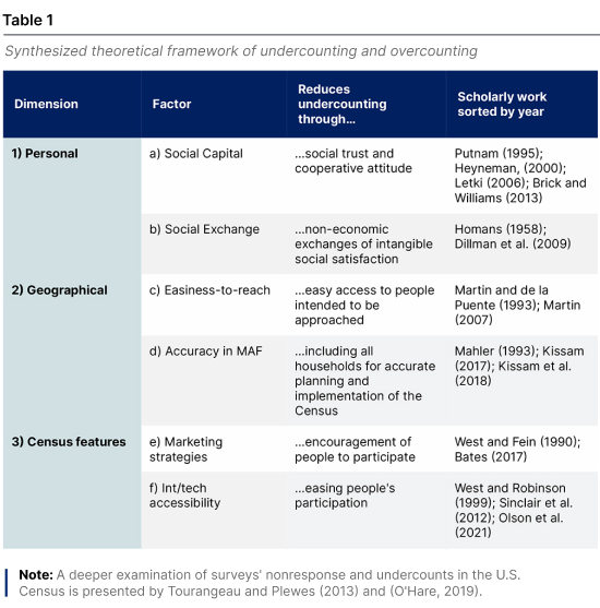 The literature around undercounting can be synthesized in a three-dimensional space, in which U&O is a function dependent on three main types of variables: personal, geographical, and Census features. At the same time, they could overlap. Moreover, each dimension might be formed by different factors. For instance, the personal dimension might embrace aspects related to a) social capital and b) social exchange. The geographical dimension might account for c) physical easiness-to-reach people in large agglomerations and d) accuracy in the Master Address File (MAF) records. The Census features dimension considers aspects related to the census implementation, such as e) marketing strategies or f) interviewer/technological accessibility. Table 1 groups the theory around these factors and explains how each factor might be related to a more accurate Census counting.
The synthesized framework shown above provides different mechanisms through which each factor is associated with lower undercounting. Then, identifying a set of variables for these factors would let us have a comparison measure of them and the dimensions across counties. After that, we estimate an equally-weighted index with these variables to proxy the number of people undercounted in each county since the U&O data for the 2020 U.S. Census is available only for states.
3. Matching theory to data
3.1. Data
Each factor can be approximated by using indicators that capture the essence of each of them. In this regard, the data is gathered from several sources (see Table 2).
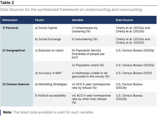 We aim to capture the essence of the Social Capital factor with a measure of social trust and cooperative attitude. With that in purpose, we lean toward the cohesiveness approach of Chetty et al. (2022a) and Chetty et al. (2022b). They define Cohesiveness as “The degree to which friendship networks are clustered into cliques and whether friendships tend to be supported by mutual friends“. Then, they measure Cohesiveness by clustering as the average fraction of an individual’s friend pairs who are also friends with each other. Theoretically, Social Exchange is envisioned as those non-economic exchanges of intangible social satisfaction across individuals. Chetty et al. (2022a) and Chetty et al. (2022b) also measure volunteering in quantifying Civic engagement. We take their Volunteering variable as it captures “the percentage of Facebook users who are members of a group which is predicted to be about ‘volunteering’ or ‘activism’ based on group title and other group characteristics“.
The Geographical dimension is composed of the Easiness-to-reach and Accuracy in MAF factors. We approximate the Easiness-to-reach dimension by using population density and population share each county represents in the state. Higher levels of population density are assumed to impose difficulties for the U.S. Census to be accurate. Similarly, large population counties would impose difficulty in counting all individuals. Another geography-related characteristic is the Accuracy of the Master Address File to identify every housing unit accurately. To measure this factor, we use the share of housing units unable to be geocoded by the U.S. Census Local Update of Census Addresses (LUCA) from the U.S. Census Bureau (2021).
The third dimension considers Census features and embraces the Marketing Strategies and Interviewer/technological accessibility factors. The first is measured using the share of the ACS 5-year housing unit nonresponse by refusal. It is expected, therefore, that higher refusal levels would increase undercounting. The second factor in this dimension is measured with the share of the ACS 5-year housing unit nonresponse by other reason than refusal U.S. Census Bureau (2022b).
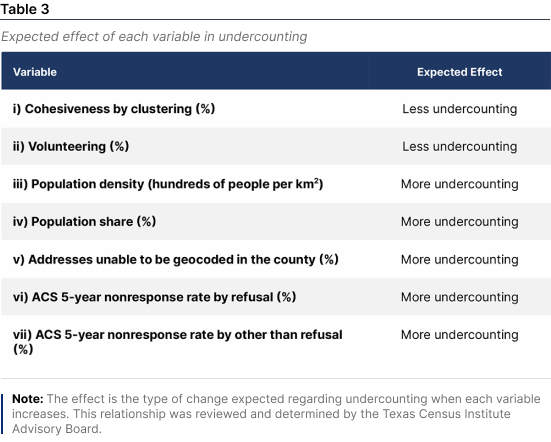 Each of the variables used here is assumed to explain the level of undercounting or overcounting in a one-way relationship. In other words, when a variable increases, it is expected to either increase the likelihood of being undercounted or decrease it, but not both. This report will present the county-level estimates for Texas. Therefore, since Texas presented an undercounting, the following sections of this report will focus on the estimation of undercounting at the county level. Table 3 presents a one-way relationship for each of the variables with undercounting.
3.2. Summary statistics
Cohesiveness by clustering and Volunteering have a “Less undercounting” relationship with undercounting. Then, they are modified to associate them directly with undercounting. Since they are percentages—on a scale from 0 to 100—a natural way to modify them is by using the distance of each of them to the maximum value. Population density is here expressed in hundreds of people per km2, which makes them have the highest of 11.45 people per km2. Since this number lies between the traditional 0 to 100 scale, we proceed with no further adjustments. The remaining variables are expressed in percentages of what they are intended to measure. Table 4 presents the summary statistics of the main variables.
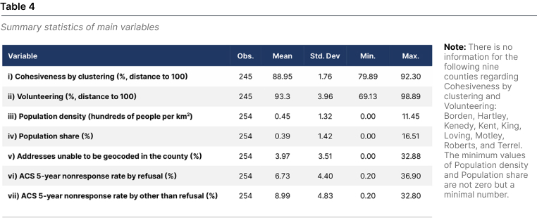
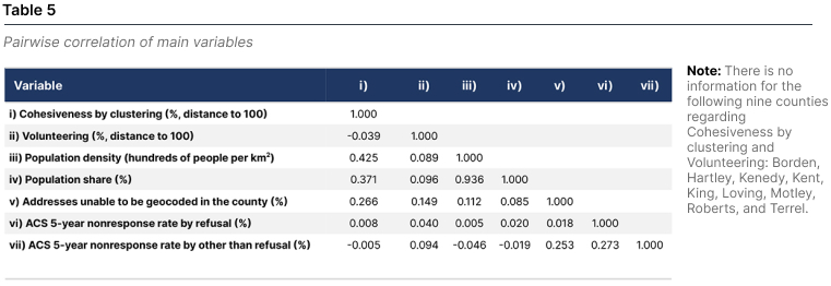
As expected, the population density and share variables are related, with a correlation coefficient of 0.9356. However, this relationship does not impose any statistical problem since both are used to measure the same Easiness-to-reach factor. The rest of the variables do not present a high correlation among them. Suggesting our selection of variables, factors, and dimensions is statistically appropriate and do not impose a substantial weight on any set of variables by double-counting them. Table 5 shows the correlation matrix of the variables used here.
4. Methodology
4.1. Measuring a county-level index for undercounting and overcounting
 The main goal of building an index for the counties is to use it to know how much of the state-level undercounting can be attributed to each county. Whatsoever, the total measure is a net value that might contain both overcounting and undercounting at the county level. Therefore, we take the 90% confidence interval of the official state-level undercounting as lower and upper bound
aries. The proportionally-weighted index proposed here would capture only undercounting for the Texas case, for which the undercounting is -1.92% with a 90% confidence interval between -3.27% and -0.57%. Due to the focus on the Texas case of undercounting, the following methodological approach takes positive terms to express undercounting and negative for overcounting. The county-level index CLI for county c in state s at year t is estimated as shown in Equation 1.
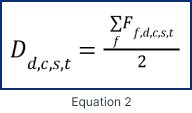 Where Dd,c,s,t is the dimension subindex for each of the dimensions d= (personal, geographical, census feature) for county c in state s at year t. It is divided by three since it is an equally-weighted index to avoid over-or under-weighting across factors. The subindex Dd,c,s,t is estimated as in Equation 2.
Where Ff,c,s,t is the average of the variables in each factor belonging to each dimension for county c in state s at year t (social capital and social exchange for the personal dimension; easiness-to-reach and accuracy in MAF for the geographical dimension; and marketing strategies and int/tech accessibility for the Census features dimension). It is divided by two since it is an equally-weighted index to avoid over-or under-weighting across factors. The original variables are standardized by dividing the difference of each value with respect to the mean by the variable’s standard deviation. This way, the original variables are first used as standard deviation units to the state mean.
4.2. Estimation of the undercounting and overcounting
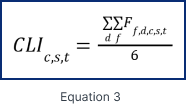 This CLIc,s,t is therefore summarizing the dimensions, which are, at the same time, embracing its factors. Then, Equation 1 and Equation 2 can be summarized as in Equation 3.
CLIc,s,t is an average of the mean-standardized version of the variables. Then, we adjust its distribution to match the official state-level undercounting. The adjustment is performed by dividing the CLIc,s,t the county-level index’s maximum (or minimum) value when it has positive (or negative) values. This allows a dispersion between -1 and 1, which is multiplied by the absolute figures of the difference between the upper and lower bounds of the 90% confidence interval and the mean undercount. Let us call it the adjusted index CLIc,s,t. Therefore, the undercount for the county c in the state s at year t is calculated as in Equation 4.
 This undercountc,s,t represents the population being undercounted when positive and overcounted when negative.
5. Results
The average county-level undercounting share is 1.52%, with a minimum of 0.46% and a maximum of 2.64%. In terms of the number of undercounted people, we found counties have an undercount of 6 to 117,073, with an average undercount of 2,237 people by county. Table 6 presents the main summary statistics.

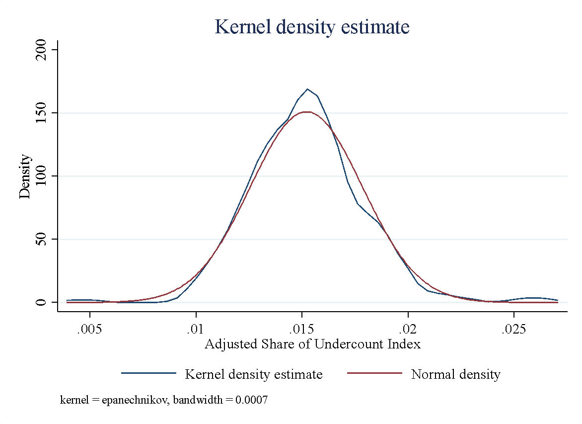
Figure 1 presents the distribution for the county-level undercounting share and (the log of) undercounting estimates in Panel a) and Panel b), respectively. Both panels show that our estimates are not skewed. It is important to emphasize that the mean and 90% confidence interval from the official U.S. Census Bureau undercounting state-level estimates are used first to estimate our undercounting share measure. Then, the distribution of our estimates might be considered moderate—or conservative—since the real undercounting at the county level might go out of the 90% confidence interval.
a)
b)
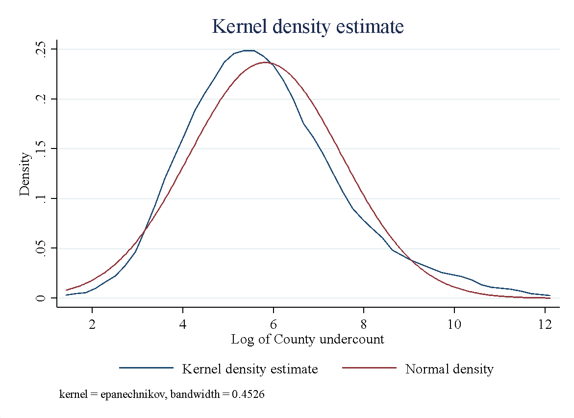
Figure 1 Distribution of the undercounting share and undercounting in Texas’ counties.
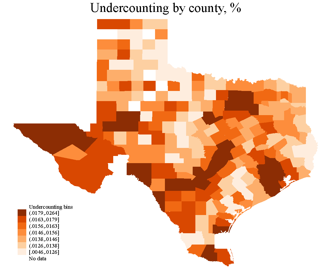
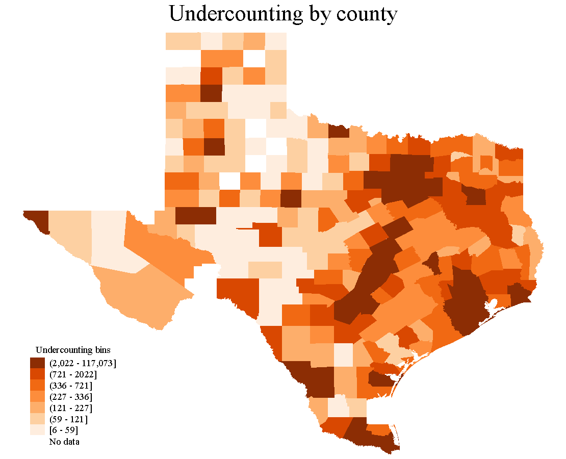
Figure 2 presents the geographical distribution of undercounting across the 245 counties with available data for all the variables. Panels a) and b) in Figure 2 present each county’s undercounting percentage and total values, respectively. The maps present seven bins for their colors. At first sight, Panel a) in Figure 2 depicts darker colors in densely populated areas (such as those of Austin, Dallas, Houston, and San Antonio) and the U.S.-Mexico border. This suggests that the intensity of undercounting (expressed in percentage terms) is higher in those areas. On the other hand, when studying the counties’ undercounting estimates, Panel b) presents a different story. As intuitively expected, Panel b) in Figure 2 shows how undercounting is higher in volume terms in highly populated counties and just a few counties on the U.S.-Mexico border.
a)

b)

Figure 2 Geographical dispersion of the undercounting share and undercounting in Texas.
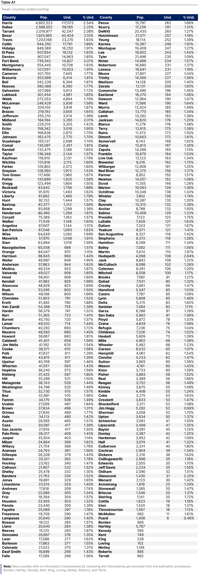
Table 7 presents the names and values of the top and bottom 20 counties in terms of undercounting. This table confirms the intense undercounting in the Austin (Travis, Williamson, Bell, and McLennan counties), Dallas (Dallas, Tarrant, Collin, and Denton), Houston (Harris, Fort Bend, Montgomery, Brazoria, and Galveston counties, and San Antonio (Bexar County) areas, and in those counties located in the U.S.-Mexico border—which also have a high undercounting in terms of population.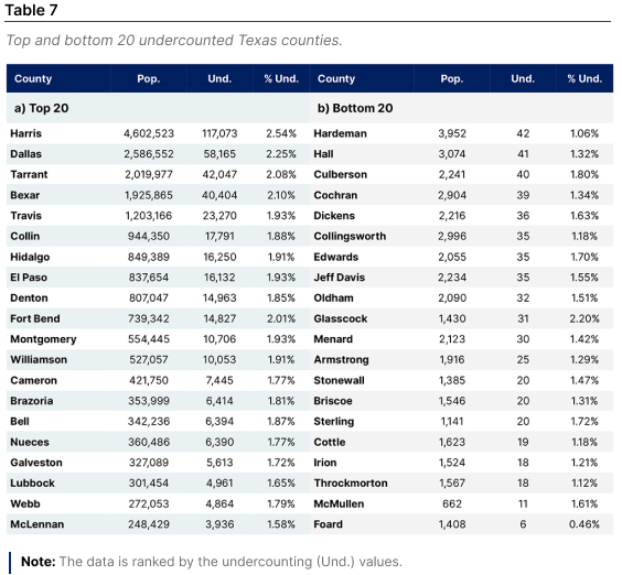 For instance, some of the counties in the U.S-Mexico border presenting darker color in both maps are El Paso, Hidalgo, Cameron, and Webb counties (where famous border cities such as El Paso, McAllen, Laredo, and Brownsville are located, respectively). In summary, from the Top-20 undercounted counties, 14 are part of large metropolitan areas, and 4 are on the U.S.-Mexico border. The other two counties, Lubbock and Webb, are located in the north and south of Texas, respectively.
The conjunct analysis of the maps in Figure 2 and lists in Table 7 allows us to observe why we should not rely only on one of the maps or on one of the extremes of the list when counties are ranked. For example, Culberson County (the third county from left to right in the maps) has remarkably different colors in the two panels, and Table 7 helps us clarify why. Culberson county has a relatively high share of undercounting (1.80%), but only 40 people were undercounted.
5.1. County-level correlations
This subsection provides an overview of the correlation of our estimates to its original theoretical determinants and relevant socioeconomic variables. The former analysis will help us identify whether our estimates are disproportionately accounted for, regardless of their proportional weights and if some of the variables exert a significant role in explaining undercounting. The latter analysis might help us understand the social and economic features surrounding undercounting.
 As a starting point, the correlation between the undercounting share and the seven original variables lies between 0.45 and 0.59. The similar correlation of the seven variables to the share of undercounting provides evidence in favor of the robustness of our approach in using variables almost equally crucial in determining undercounting. However, interpreting the correlation coefficients between the estimated undercounted people by county and the seven original variables must be taken with caution since the estimate of undercounted people is the product of counties’ population and the share of undercounting. Therefore, the estimated undercounted population will automatically correlate with the counties’ population share (0.99) and population density (0.90). Interestingly, the estimate of undercounted people is not related to four of the other five variables (volunteering, addresses unable to be geocoded in the county, ACS 5-year nonresponse rate by refusal, and ACS 5-year nonresponse rate by other than refusal) with correlation coefficients from -0.01 to 0.09; but slightly—if something—related to the Cohesiveness by clustering variable, with a correlation coefficient of 0.33.
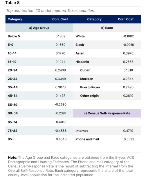
The methodological approach presented is limited to the availability of reliable data at the county level for each of the seven theoretical determinants. Therefore, to further assess the relationship of the county-level undercounting to demographic characteristics and the Census implementation. Correlation coefficients are estimated for different population categories according to age, race, and the Census response method (see Table 8).
Panel a) in Table 8 shows that the share of people in groups below 54 years old is positively associated with higher undercounting, and groups above 55 years and older are negatively associated with undercounting. These findings might reflect the relevance and participation given to the Census by older groups of people. Similarly, this might arise since younger population groups are more likely to be part of the labor force and not to be available to respond to the Census or to be counted appropriately. The population groups below 54 years present an inverse-U relationship to undercounting, with its maximum correlation estimate for those 25-34 years old (0.3349). On the other hand, the negative relationship to undercounting increases as population groups get older, with its maximum in the 75-84 group (-0.4566). These results are robust to those presented by the Census Demographic Analysis in which younger groups are associated with undercounting, and older groups above are inversely related to it (Jensen & Kennel, 2022).
Regarding racial categories, the share of white people is negatively related to the counties’ undercounting share, with a correlation coefficient of -0.1802. Suggesting that white people might be less likely to be undercounted. The share of the Black population in the counties is technically not related to undercounting, with a correlation estimate of -0.0018. On the other hand, the Asian and Hispanic population’s shares are positively associated with a higher undercounting share, with a correlation coefficient of 0.3970 and 0.2566, respectively. When studying the Hispanic population, the share of those not from Puerto Rico, Cuba, or Mexico is associated with a higher counties’ undercounting share (0.2619)—closely followed by Puerto Rico and Mexico, with correlation coefficients of 0.2420 and 0.2340. The correlation between our undercounting shares and racial groups coincides with those of the Census Post-Enumeration Survey, in which the Hispanic population is associated with higher undercounting, and the white population has the opposite relationship (Jensen & Kennel, 2022).
Our estimates can also be compared to the self-response rates of the 2020 U.S. Census. In this regard, it is important to signal that the last Census was the first one in which it was implemented via the Internet (Bates, 2017). Our county-level undercounting share has a strong and positive correlation coefficient to the share of people that self-responded via the Internet (0.4719) and a strong and negative value with the share that self-responded via traditional methods, such as telephone and mail (-0.5522). While these findings unveil some plausible risks from implementing the Census online, we encourage the reader to take this with caution since a causal statement should not arise from this analysis. Instead, we encourage future research lines to study the causal mechanisms driving the undercounting and overcounting in the United States.
6. Concluding remarks
In this report, we propose a practical methodology to estimate Census undercounting at the county level and present its main results for Texas and Texas’ population groups—categorized by age, race, and Census self-response method. To do so, we account for personal, geographical, and Census features dimensions to first build a theory-based model with determinants of undercounting. Then, we estimate a proportionally-weighted index to allocate counties along the 90% confidence interval of the state-level undercounting provided by the Census.
Texas’ estimates suggest intense undercounting—in terms of undercounting share—occurs in the Austin (Travis, Williamson, Bell, and McLennan counties), Dallas (Dallas, Tarrant, Collin, and Denton), Houston (Harris, Fort Bend, Montgomery, Brazoria, and Galveston counties, and San Antonio (Bexar County) areas. Moreover, undercounting is observed in those counties located on the U.S.-Mexico border (El Paso, Hidalgo, Cameron, and Webb County, where El Paso, McAllen, Laredo, and Brownsville are located)—which also have a high undercounting in terms of population.
The county-level dynamics across age groups and race categories suggest this approach is robust to the overall dynamics found by the U.S. Census Demographic Analysis and Post-Enumeration Survey. Our analysis suggests that the share of the population in younger groups is associated with higher undercounting and that the share of older groups is inversely related to undercounting. We also find that the counties’ share of white people is inversely associated with undercounting, and the share of the Hispanic population is associated with higher levels of undercounting. Moreover, we identified a positive relationship between the counties’ Census self-response rates via the Internet and our estimates of the share of undercounting, which might be the result of undercounting occurring in counties where the access to the Internet is limited or just of the lack of strong participation of people via the Internet. Our theory-based approach aims to be a cornerstone in the alternative estimation of undercounting and overcounting. More research is recommended to obtain a comprehensive understanding of undercounting and overcounting.
Authors Message
To the extent that counties might present undercounting and overcounting approximations, their estimates might be different due to unobservable reasons. However, even in these circumstances, our undercounting and overcounting approximations aim to be a sufficient guide for intervention. The general goal of our methodology is to provide a data-driven exploration of what Texans are counted or not and to pursue ideas for creating an equitable census.
Acknowledgements: The authors appreciate the insightful support provided by Dr. Lloyd B. Potter, Dr. Monica Cruz, Dr. Mary Campbell, and Dr. Shannon Cavanagh.
FAQ
1) Why does the U.S. Census Bureau not publish undercounting and overcounting estimates at the county level?
The official answer is that “Given the sample size for the 2020 [Post-Enumeration Survey] (PES) and the assumptions required to make unbiased sub-state estimates, the Census Bureau was unable to include county or place estimates in the 2020 PES reports, as well.” (U.S. Census Bureau, 2022) .
2) What does a “Determinants-Side Approach” mean in this context?
This approach implies that undercounting estimation is built upon variables that are considered determinants of undercounting, according to the theory.
3) How accurate or precise are our undercounting estimates?
There is no statistical measure of accuracy or precision for our estimates. However, they are considered conservative measures since they allow the counties to have an undercounting share within the 90% confidence level interval of the state-level undercounting.
4) Why are we considering individual, geographical, and census features as criteria for calculating the undercount?
We recognize that undercounting might arise from basic elements of counting population: each person itself, its natural environment, and the mechanism used to count. Therefore, parsimony makes it straightforward to identify undercounting determinants coming from each of these criteria.
5) Why do we not use variables associated with demographic characteristics?
We have not found theoretical evidence that any demographic characteristic is a singular determinant of undercounting. While some specific population groups are believed to be undercounted, it is not due to their demographic characteristics alone, but more accurately attributed to their individual, geographical and census features.
